Finding and Plotting Solar Orbiter MAG Data

This example demonstrates how to search for, download, and visualize 1-minute averaged Solar Orbiter MAG (Magnetometer) data from the SOAR archive, load it into a SunPy TimeSeries, and plot it.

import matplotlib.pyplot as plt
from sunpy.net import Fido, attrs as a
import sunpy_soar
from sunpy.timeseries import TimeSeries as ts

By importing sunpy_soar, the Solar Orbiter Archive (SOAR) is automatically registered as a data provider in Fido. This allows us to directly query and download Solar Orbiter data just like any other SunPy Fido search.

Now, we will use Fido to search for MAG Level 2 data in Radial-Tangential-Normal (RTN) coordinates. We will request 1-minute averaged data over a two-day period.

search_results = Fido.search(
    a.Time("2022-09-04", "2022-09-06 00:00"),
    a.Instrument.mag,
    a.soar.Product('mag-rtn-normal-1-minute'),
    a.Level(2)
)

print(search_results)

Results from 1 Provider:

3 Results from the SOARClient:

Instrument       Data product      Level        Start time               End time        Filesize SOOP Name
                                                                                          Mbyte
---------- ----------------------- ----- ----------------------- ----------------------- -------- ---------
       MAG mag-rtn-normal-1-minute    L2 2022-09-04 00:00:00.000 2022-09-05 00:00:00.000    0.033      None
       MAG mag-rtn-normal-1-minute    L2 2022-09-05 00:00:00.000 2022-09-06 00:00:00.000    0.033      None
       MAG mag-rtn-normal-1-minute    L2 2022-09-06 00:00:00.000 2022-09-07 00:00:00.000    0.033      None

The search results contain a list of available files matching our query. We use Fido.fetch to download the files.

downloaded_files = Fido.fetch(search_results)

Files Downloaded:   0%|          | 0/3 [00:00<?, ?file/s]

solo_L2_mag-rtn-normal-1-minute_20220904_V02.cdf:   0%|          | 0.00/32.8k [00:00<?, ?B/s]


solo_L2_mag-rtn-normal-1-minute_20220905_V02.cdf:   0%|          | 0.00/32.6k [00:00<?, ?B/s]



solo_L2_mag-rtn-normal-1-minute_20220906_V02.cdf:   0%|          | 0.00/32.7k [00:00<?, ?B/s]

solo_L2_mag-rtn-normal-1-minute_20220904_V02.cdf:   3%|▎         | 1.02k/32.8k [00:00<00:06, 5.23kB/s]


solo_L2_mag-rtn-normal-1-minute_20220905_V02.cdf:   3%|▎         | 888/32.6k [00:00<00:07, 4.36kB/s]



solo_L2_mag-rtn-normal-1-minute_20220906_V02.cdf:   3%|▎         | 1.02k/32.7k [00:00<00:06, 5.04kB/s]

solo_L2_mag-rtn-normal-1-minute_20220904_V02.cdf:  45%|████▍     | 14.7k/32.8k [00:00<00:00, 59.9kB/s]


solo_L2_mag-rtn-normal-1-minute_20220905_V02.cdf:  45%|████▌     | 14.7k/32.6k [00:00<00:00, 57.3kB/s]



solo_L2_mag-rtn-normal-1-minute_20220906_V02.cdf:  45%|████▍     | 14.7k/32.7k [00:00<00:00, 57.2kB/s]

solo_L2_mag-rtn-normal-1-minute_20220904_V02.cdf: 100%|██████████| 32.8k/32.8k [00:00<00:00, 104kB/s]


Files Downloaded:  33%|███▎      | 1/3 [00:00<00:01,  1.19file/s]


solo_L2_mag-rtn-normal-1-minute_20220905_V02.cdf:  99%|█████████▊| 32.2k/32.6k [00:00<00:00, 96.4kB/s]






solo_L2_mag-rtn-normal-1-minute_20220906_V02.cdf: 100%|██████████| 32.7k/32.7k [00:00<00:00, 98.3kB/s]




Files Downloaded: 100%|██████████| 3/3 [00:00<00:00,  3.46file/s]

Loading the MAG Data into a SunPy TimeSeries

The downloaded file contains time-series magnetic field measurements. We use sunpy.timeseries.TimeSeries to load and analyse the data.

The concatenate=True argument ensures that if multiple files are downloaded, they are combined into a single continuous TimeSeries object.

mag_ts = ts(downloaded_files, concatenate=True)

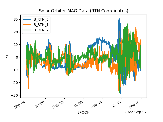
Plotting the Magnetic Field Components

We now plot these components over time.

mag_ts.plot(columns=["B_RTN_0", "B_RTN_1", "B_RTN_2"])

plt.title("Solar Orbiter MAG Data (RTN Coordinates)")
plt.show()